
§1. Introduction
The Over-Parameterization Dilemma in Medical AI
Artificial intelligence, especially deep learning, has transformed modern computing. However, this predictive power comes at a severe computational cost. Models like VGG19 require massive parameter budgets, creating serious deployment barriers for edge-AI devices, embedded platforms, and point-of-care medical hardware.
Theoretical Foundations & Literature Context
Classical statistical learning theory suggests highly over-parameterized models should overfit badly. Modern deep learning departs from this via benign overfitting and double descent. Post-training compression acts as a crucial engineering step to capture sparse active subnetworks.
§2. Research Methodology
Neural Networks as Statistical Composition Models
We reframe deep neural networks as highly parameterized compositions of Generalized Linear Models (GLMs). Unlike classical linear regressions with fixed functional forms, a neural network learns representation transitions directly from high-dimensional input spaces.
Empirical Risk & Categorical Log-Likelihood
Training minimizes an empirical risk functional over the observed sample. For multi-class diagnostics, this is equivalent to minimizing the negative log-likelihood of a multinomial model.
2.3 Dataset: BloodMNIST
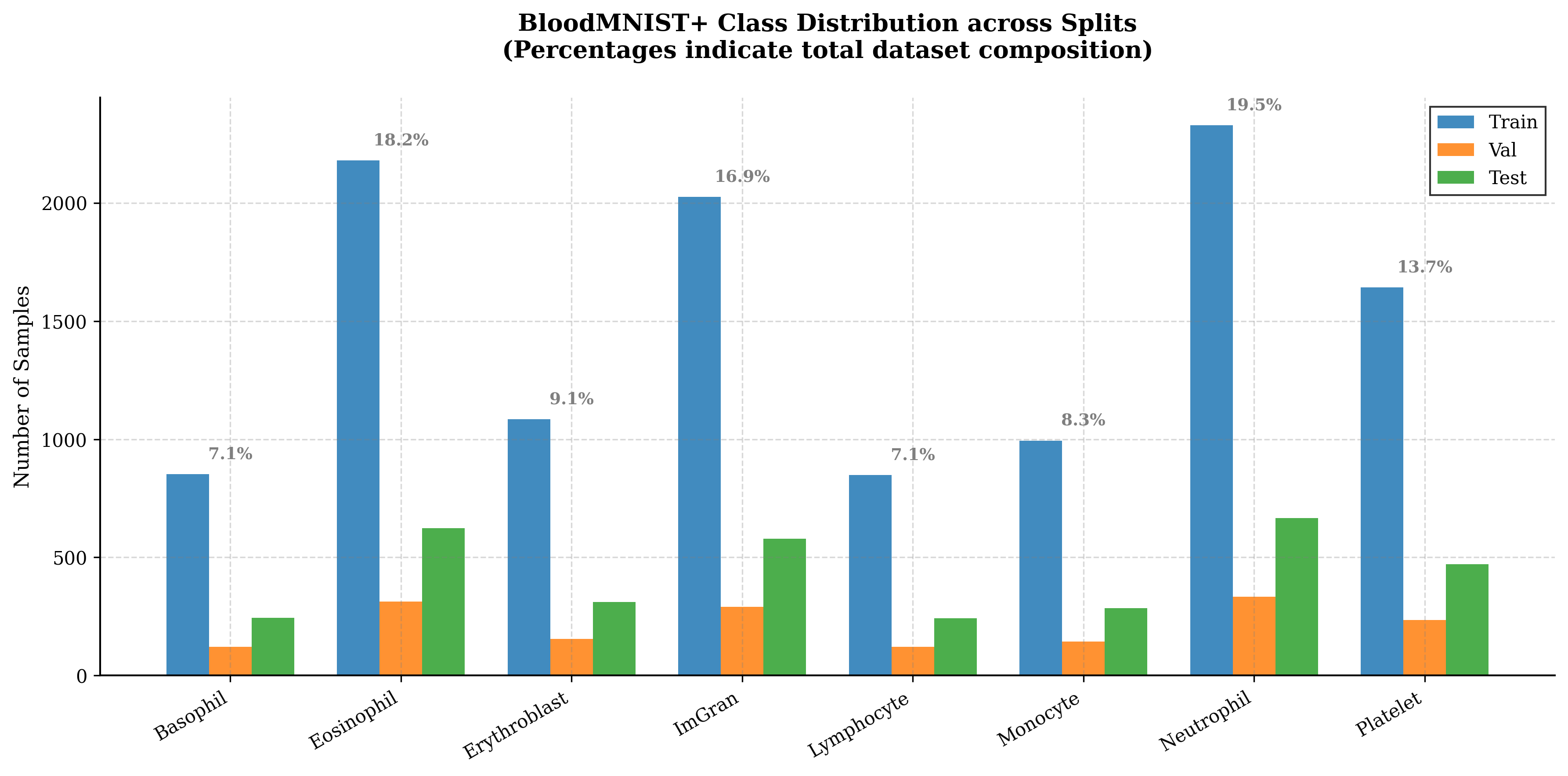
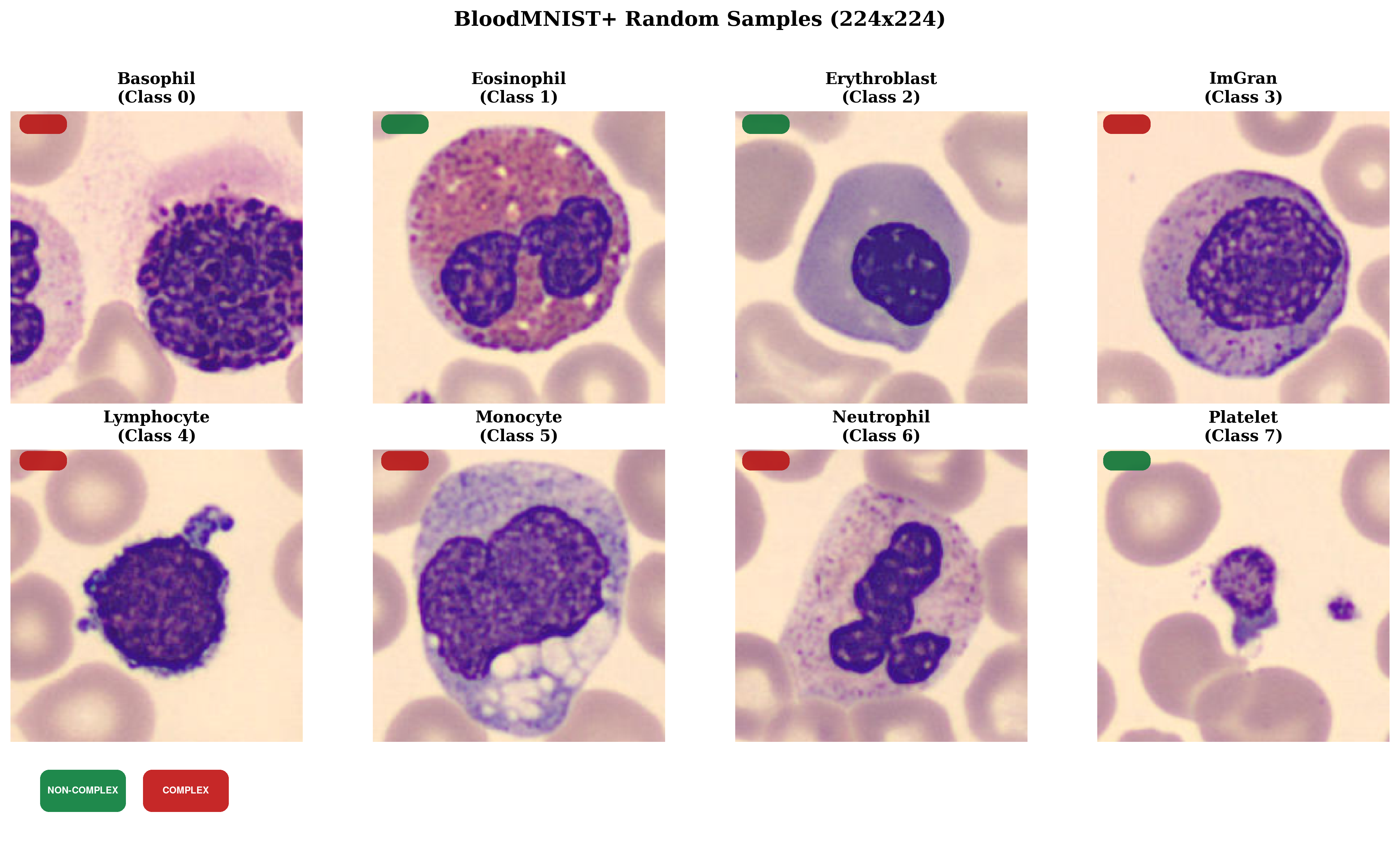
We use the BloodMNIST dataset from the MedMNIST benchmark family, containing 17,092 labelled peripheral blood-cell images across eight diagnostic classes.
Scientific Observation Table
| Cell Class | Train | Val | Test | Total | Share |
|---|---|---|---|---|---|
| Basophil | 852 | 122 | 244 | 1,218 | 7.13% |
| Eosinophil | 2,181 | 312 | 624 | 3,117 | 18.24% |
| Erythroblast | 1,085 | 155 | 311 | 1,551 | 9.07% |
| Immature Granulocytes | 2,026 | 290 | 579 | 2,895 | 16.94% |
| Lymphocyte | 849 | 122 | 243 | 1,214 | 7.10% |
| Monocyte | 993 | 143 | 284 | 1,420 | 8.31% |
| Neutrophil | 2,330 | 333 | 666 | 3,329 | 19.48% |
| Platelet | 1,643 | 235 | 470 | 2,348 | 13.74% |
BloodMNIST class distribution across train, validation, and test splits — Neutrophils and Eosinophils form the largest classes; Lymphocytes and Basophils the smallest. This imbalance is methodologically relevant because compression artefacts often manifest first in minority classes.
Images were normalized using standard ImageNet distribution vectors:
Centering and scaling ensures early convolutional filters operate within stable pretrained activation ranges.
Second-Order Loss Sensitivity & Optimal Pruning
Saliency metrics define weight importance by measuring empirical risk change under small weight perturbations. Under the Optimal Brain Surgeon framework, we calculate parameters' diagonal sensitivities via the inverse Hessian matrix.
Sparsity regularizers and matrix factorization rules
To physically shrink the network, we evaluate L1 Lasso unstructured penalties, continuous Gaussian relaxation of L0 gates for spatial channels, and Singular Value Decomposition (SVD) low-rank factorization.
§3. Baseline Model Analysis
Baseline Architecture & Empirical Redundancy Analysis
The uncompressed VGG19 model acts as our empirical upper bound. It contains sixteen convolutional layers and three fully connected layers, encompassing 139.6 million learnable parameters—exhibiting extreme redundancy for an 8-class diagnostic task.
Fine-Tuning Protocol & Convergence Dynamics
We initialize VGG19 with pretrained ImageNet weights and fine-tune using SGD with Nesterov momentum. Training converges within 15 epochs, capturing high-quality hematological representation states.
Empirical Layer Activation PCA Redundancy Audit
Principal component decomposition of intermediate activations, verifying feature-space dimensionality reduction.
Convolutional Block 5 Activations
The highest spatial layers show a rapid decay in active dimensions. Despite a capacity of 512 channels, the feature representations occupy a highly restricted subspace of only 59 components (88.5% redundant). This rapid collapse confirms that late spatial features reside on an extremely low-dimensional manifold.
For layer activation matrix H, Singular Value Decomposition isolates orthogonal feature eigenvectors. The parsimonious subspace rank k is selected under an energy cutoff η = 0.95:
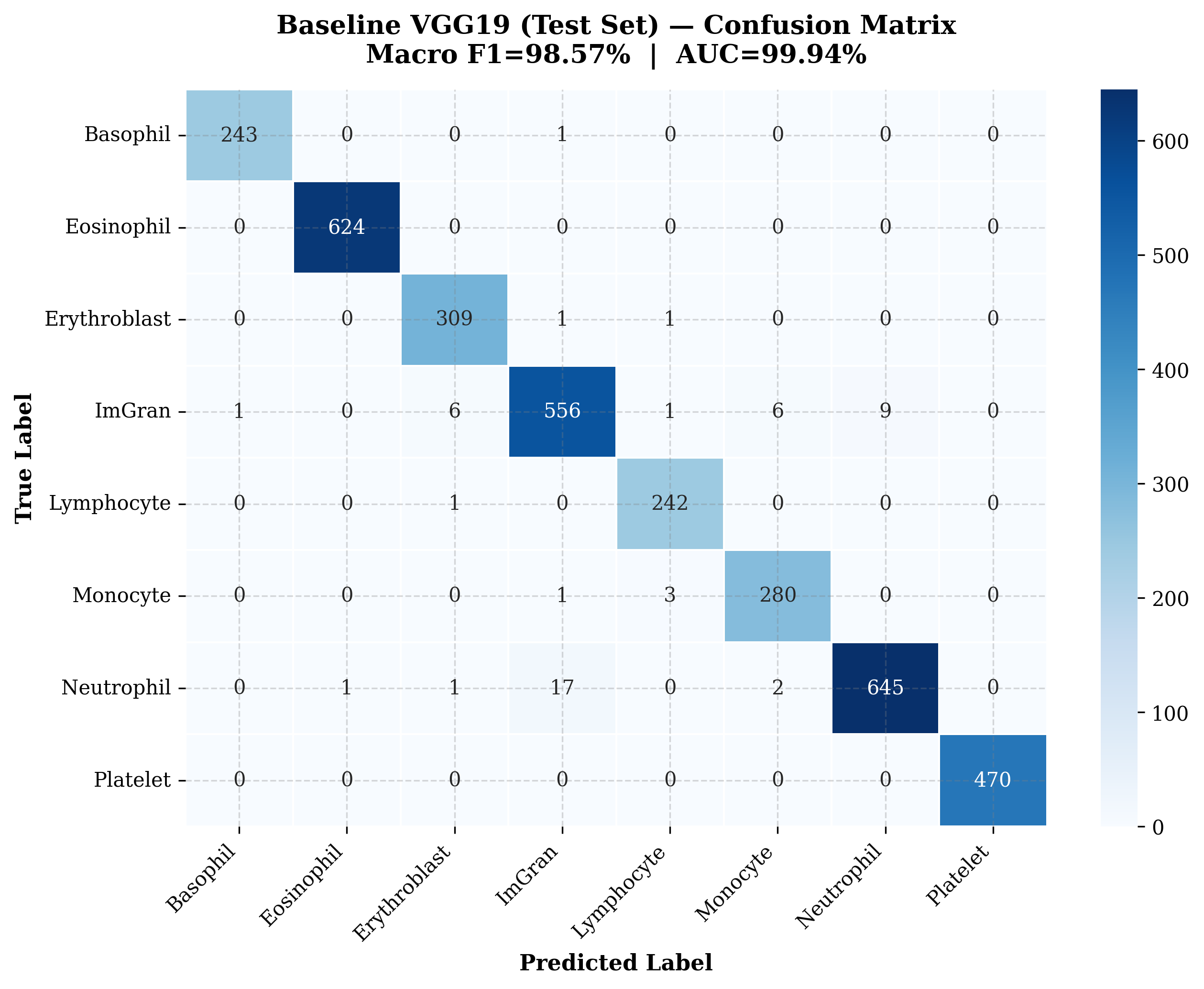
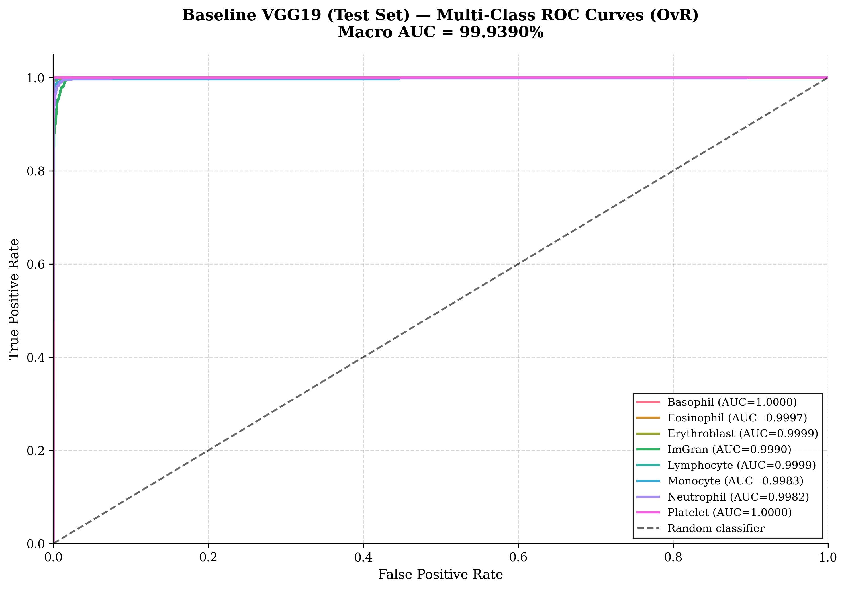
3.4 Diagnostic Performance Summary
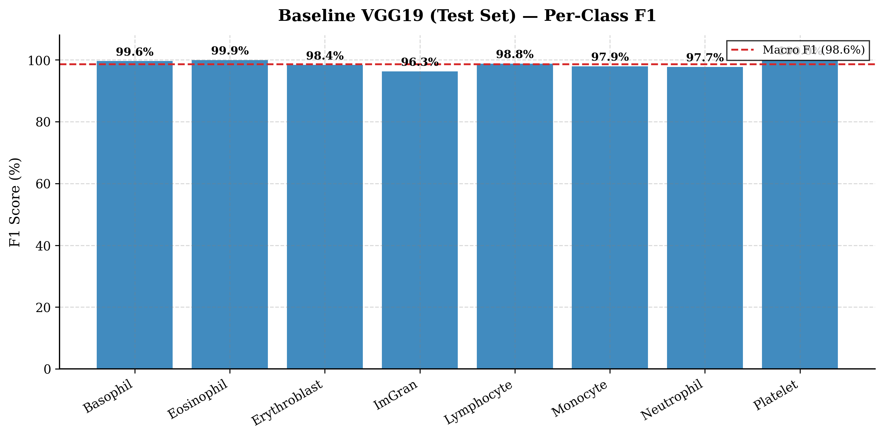
Evaluated on the blind test set (Ntest = 3,421), the baseline model sets a high clinical standard:
Scientific Observation Table
| Cell Class | Support | Precision | Recall | F1 | Accuracy |
|---|---|---|---|---|---|
| Basophil | 244 | 99.59% | 99.59% | 99.59% | 99.97% |
| Eosinophil | 624 | 99.84% | 99.84% | 100.00% | 99.96% |
| Erythroblast | 311 | 98.41% | 97.48% | 99.36% | 99.74% |
| Immature Gran. | 579 | 96.28% | 96.53% | 96.03% | 99.30% |
| Lymphocyte | 243 | 98.78% | 97.98% | 99.59% | 99.84% |
| Monocyte | 284 | 97.90% | 97.22% | 98.59% | 99.74% |
| Neutrophil | 666 | 97.73% | 98.62% | 96.85% | 99.67% |
| Platelet | 470 | 100.00% | 100.00% | 100.00% | 100.00% |
Class-wise diagnostic performance of the baseline VGG19 — Minimum F1 in Immature Granulocytes (96.28%)—a continuous developmental lineage with high morphological variance.
3.5 Computational Complexity & Resource Demand
Despite strong diagnostic accuracy, the model has massive deployment costs:
The extreme AIC and BIC scores confirm that VGG19 is massively over-parameterized for this 8-class diagnostic task. This structural redundancy motivatess our statistical compression study.
§4. L1 Lasso Regularization
L1 Shrinkage Penalty & Experimental Setup
We first evaluate L1 Lasso as the simplest sparsity-inducing mechanism. The classification cross-entropy loss is augmented with a penalty that forces minor parameters toward zero, producing unstructured sparsity.
Training Dynamics & Phase Transition Collapse
We document a major phase transition at epoch 22. The cumulative pressure of L1 regularizers overwhelmed model representational capacity, causing validation performance to collapse. We recover the stable epoch 20 state.
Iterative Magnitude Pruning (IMP) & Refinement
Three cycles of iterative magnitude pruning (IMP) and weight masking convert soft L1 shrinkage parameters into true hard zeros, creating a light uncompressed network mask.
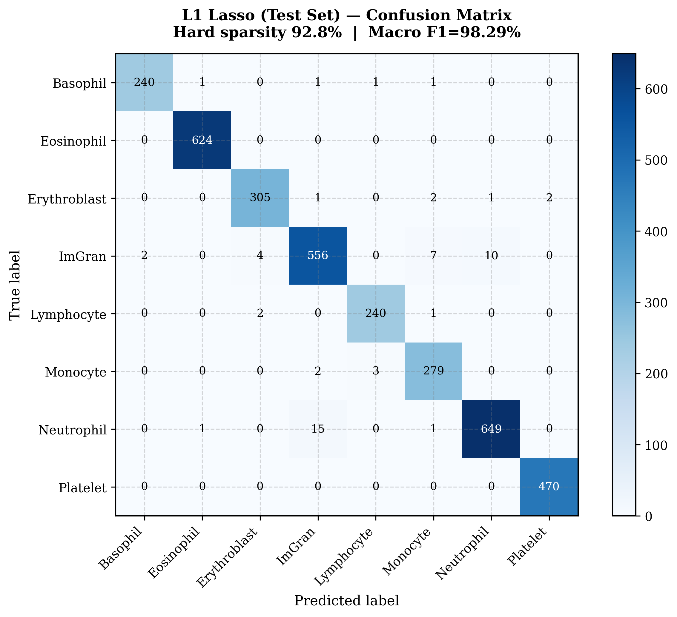
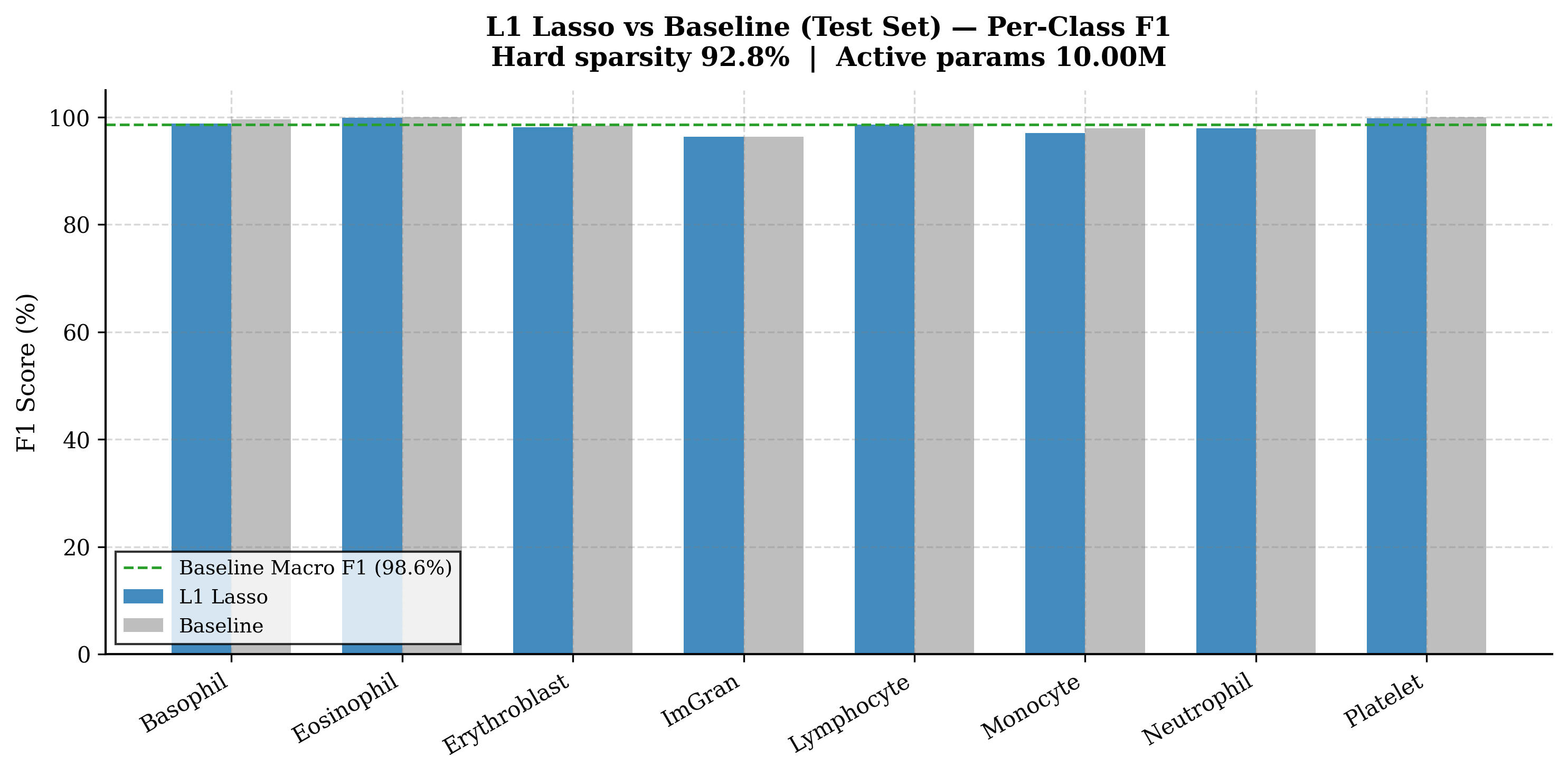
4.4 Diagnostic Performance Verification
Evaluated on the blind test set, the final L1-pruned network preserves macro-F1 at 98.29% (−0.28 pp baseline penalty):
Scientific Observation Table
| Cell Class | Baseline F1 | L1 F1 | Δ F1 | Base Recall | L1 Recall |
|---|---|---|---|---|---|
| Basophil | 99.59% | 98.77% | −0.82% | 99.17% | 98.36% |
| Eosinophil | 99.92% | 99.84% | −0.08% | 99.68% | 100.00% |
| Erythroblast | 98.41% | 98.07% | −0.34% | 98.07% | 98.07% |
| Immature Gran. | 96.28% | 96.36% | +0.08% | 96.70% | 96.03% |
| Lymphocyte | 98.78% | 98.56% | −0.22% | 98.36% | 98.77% |
| Monocyte | 97.90% | 97.04% | −0.86% | 95.88% | 98.24% |
| Neutrophil | 97.73% | 97.89% | +0.16% | 98.33% | 97.45% |
| Platelet | 100.00% | 99.79% | −0.21% | 99.58% | 100.00% |
Class-wise comparison: Baseline vs L1 Lasso — Even Immature Granulocytes retained F1 = 96.36%, above the 90% clinical guardrail.
4.5 L1 Complexity & Unstructured Profile
Critical Finding: Ghost Sparsity Paradox
Despite eliminating 129.6M parameters (92.8% sparsity), physical inference latency increased to 207.0 ± 15.2 ms per batch—slower than the uncompressed baseline. GPU memory expanded to 4,854.0 MB.
Because L₁ zeros individual weights at random locations (unstructured sparsity), the physical tensor dimensions remain unchanged. Standard deep learning libraries still calculate matrix multiplications over these zeros. This “ghost sparsity” paradox proves that unstructured sparsity does not deliver real-world hardware speedups on standard GPUs, motivating our shift to structured channel pruning.
Information-theoretically, L1 was highly successful: AIC dropped from 2.79×10⁸ to 2.00×10⁷, and BIC to 8.13×10⁷. However, this statistical parsimony did not translate to faster inference. This motivates our shift toward structurally enforced compression methods.
§5. L0 Gaussian Gating & Tensor Surgery
5.1 PCA Redundancy Audit
Before introducing structural gates, activation PCA measured exact representation redundancy under a 95% variance threshold:
Scientific Observation Table
| Layer | Total Dims | Dims for 95% Var | Redundancy |
|---|---|---|---|
| Conv Block 3 | 256 | 41 | 84.0% |
| Conv Block 4 | 512 | 122 | 76.2% |
| Conv Block 5 | 512 | 59 | 88.5% |
| FC0 activations | 4,096 | 285 | 93.0% |
| FC3 activations | 4,096 | 137 | 96.7% |
PCA redundancy audit for baseline VGG19 — Split strategy: Truncated SVD for linear classification layers, L0 structured gating for convolutional filter base.
Hard Concrete Optimization Failure & The Gaussian Pivot
Six separate training runs using Hard Concrete discrete estimators failed to close convolutional gates (sparsity remained at 0.0%). We pivot to a continuous Gaussian approximation, enabling smooth backpropagation.
PID-Controlled Sparsity Target Stabilization
To target a physical 60% channel sparsity without destabilizing classification performance, we integrate a PID controller that modulates regularization strength dynamically.
5.4 Layer-wise Survival Profile
The selected checkpoint achieves 69.1% gate sparsity and 74.5% weight sparsity. Convolutional layers show a strong depth-dependent survival gradient:
Scientific Observation Table
| Layer | Block | Total Ch. | Open | Closed | Survival |
|---|---|---|---|---|---|
| L1 | Conv Block 1 | 64 | 40 | 24 | 62.5% |
| L2 | Conv Block 1 | 64 | 47 | 17 | 73.4% |
| L3 | Conv Block 2 | 128 | 97 | 31 | 75.8% |
| L4 | Conv Block 2 | 128 | 112 | 16 | 87.5% |
| L5 | Conv Block 3 | 256 | 122 | 134 | 47.7% |
| L6 | Conv Block 3 | 256 | 116 | 140 | 45.3% |
| L7 | Conv Block 3 | 256 | 127 | 129 | 49.6% |
| L8 | Conv Block 4 | 256 | 133 | 123 | 52.0% |
| L9 | Conv Block 4 | 512 | 115 | 397 | 22.5% |
| L10 | Conv Block 4 | 512 | 112 | 400 | 21.9% |
| L11 | Conv Block 4 | 512 | 123 | 389 | 24.0% |
| L12 | Conv Block 4 | 512 | 124 | 388 | 24.2% |
| L13 | Conv Block 5 | 512 | 114 | 398 | 22.3% |
| L14 | Conv Block 5 | 512 | 97 | 415 | 18.9% |
| L15 | Conv Block 5 | 512 | 110 | 402 | 21.5% |
| L16 | Conv Block 5 | 512 | 83 | 429 | 16.2% |
Per-layer gate survival after L0 training in the VGG19 convolutional base — Total: 4,896 channels → 1,572 surviving (32.1% open / 67.9% pruned). Early blocks preserve edge and color features; deep blocks shed high-dimensional ImageNet-specific filters.
From Masked Complexity to Physical Tensor Surgery
An active gate mask does not yield physical speedup on standard GPUs due to dense masking multiplication overhead. We perform hardware tensor surgery, physically slicing surviving channels into a smaller dense architecture.
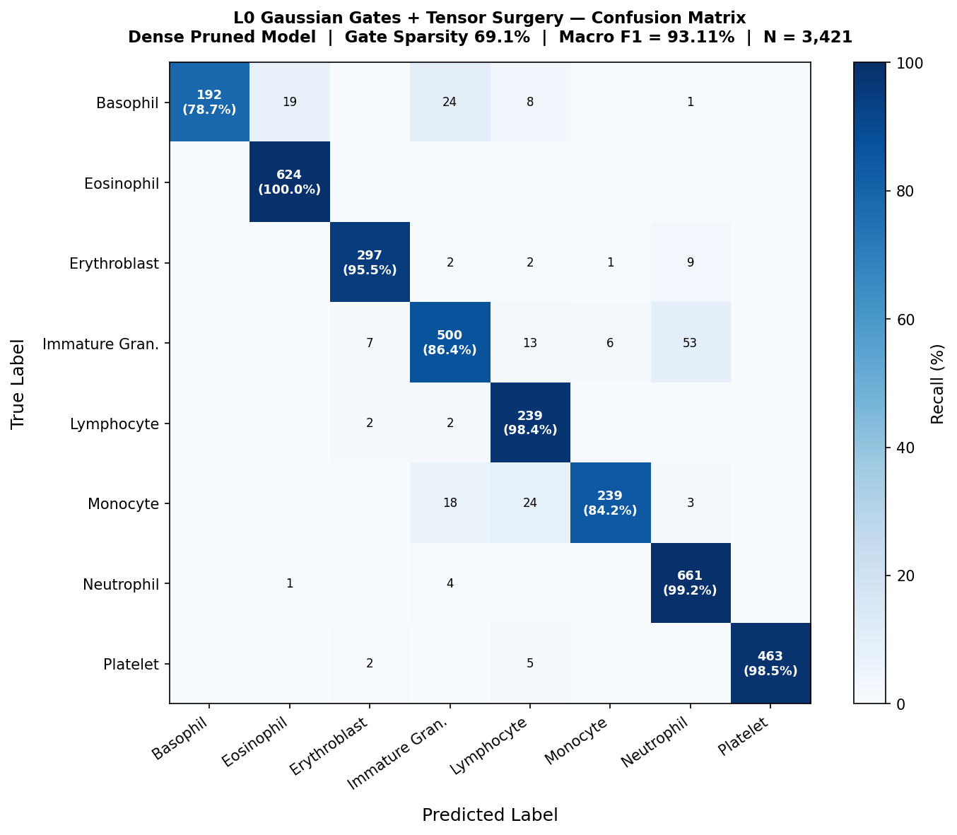
5.6 Clinical Diagnostic Performance Comparison
Scientific Observation Table
| Cell Class | Support | F1 | Precision | Recall | AUC | Δ F1 |
|---|---|---|---|---|---|---|
| Basophil | 244 | 88.07% | 100.00% | 78.69% | 99.84% | −11.52% |
| Eosinophil | 624 | 98.42% | 96.89% | 100.00% | 99.98% | −1.50% |
| Erythroblast | 311 | 95.96% | 96.43% | 95.50% | 99.53% | −3.54% |
| Immature Gran. | 579 | 88.57% | 90.91% | 86.36% | 99.01% | −8.00% |
| Lymphocyte | 243 | 89.51% | 82.13% | 98.35% | 99.81% | −9.90% |
| Monocyte | 284 | 90.19% | 97.15% | 84.15% | 99.47% | −8.40% |
| Neutrophil | 666 | 94.90% | 90.92% | 99.25% | 99.79% | −3.60% |
| Platelet | 470 | 99.25% | 100.00% | 98.51% | 100.00% | −0.75% |
L0 per-class performance vs baseline — All classes remain above the 85% clinical guardrail. Reductions are concentrated in Basophils (-11.52%) and Lymphocytes (-9.90%).
5.7 Hardware Surgery Outcomes
§6. Singular Value Decomposition (SVD)
FC Saliency Factorization & Matrix Dimensionality
L1 Lasso demonstrated representation redundancy but failed to accelerate physical hardware. SVD targets the structural dimensionality of fully connected layers, which account for 89% of VGG19's total parameter count.
Optimal Rank Energy Threshold Sweep
An energy threshold sweep on the validation partition identified the optimal truncation rank, exposing a sharp representational phase transition between energy coefficients 0.20 and 0.10.
Joint Adaptation Fine-Tuning & Noise Filtration
The truncated low-rank network underwent a 10-epoch joint adaptation cycle with the convolutional base frozen. By epoch 4, validation macro-F1 already surpassed the uncompressed baseline.
6.4 Blind Test Set Generalization Verification
Evaluated on the blind test set, the SVD model achieved 98.77% macro-F1, actually improving on the uncompressed baseline (+0.20 pp):
Scientific Observation Table
| Cell Class | Baseline F1 | SVD F1 | Δ F1 | Base Recall | SVD Recall |
|---|---|---|---|---|---|
| Basophil | 99.59% | 99.18% | −0.41% | 99.17% | 98.77% |
| Eosinophil | 99.92% | 99.84% | −0.08% | 99.68% | 100.00% |
| Erythroblast | 98.41% | 99.19% | +0.78% | 98.07% | 98.71% |
| Immature Gran. | 96.28% | 97.06% | +0.78% | 96.70% | 96.89% |
| Lymphocyte | 98.78% | 98.37% | −0.41% | 98.36% | 99.18% |
| Monocyte | 97.90% | 98.59% | +0.69% | 95.88% | 98.24% |
| Neutrophil | 97.73% | 97.98% | +0.25% | 98.33% | 98.20% |
| Platelet | 100.00% | 100.00% | 0.00% | 99.58% | 100.00% |
Class-wise comparison: Baseline vs SVD — Minimum per-class F1 improved from 96.28% (baseline) to 97.06% (IG), confirming preserved morphological boundaries.
6.5 SVD Compression & Complexity Profile
Critical Finding: SVD Latency Paradox
Despite eliminating 84.5% of parameters (and reducing fully connected FLOPs by 98.7%), inference latency increased to 208.1 ± 16.6 ms per batch—slower than the uncompressed baseline.
At extreme ranks (k = 44 and k = 31), the two sequential matrix multiplications are too small to saturate the massive parallel cores of modern GPUs. The compute pipeline shifts from being arithmetic-bound to kernel-dispatch bound. This paradox shows that physical layer compression does not guarantee physical latency speedups, motivating our shift to the convolutional layers via L0 structured pruning.
§7. Discussion & Unified Comparison
We return to our central research inquiry: can statistically grounded model compression reduce VGG19 complexity while preserving diagnostic performance? Below we present our unified empirical results:
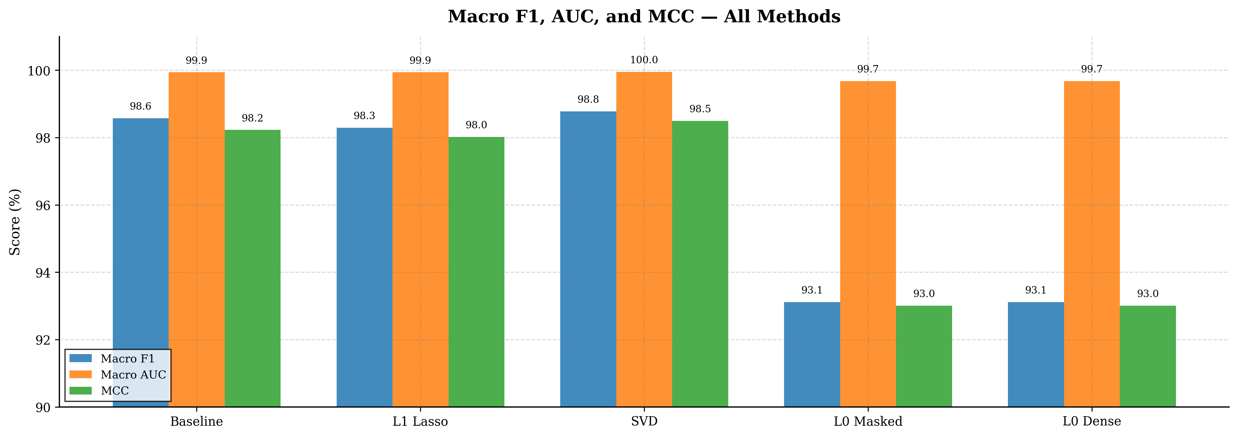
Scientific Observation Table
| Method | Top-1 Acc | Macro F1 | Δ F1 | AUC | MCC | Kappa | Loss | Min F1 |
|---|---|---|---|---|---|---|---|---|
| Baseline | 98.48% | 98.57% | — | 99.94% | 98.23% | 98.23% | 0.0488 | 96.28% |
| L₁ Lasso | 98.30% | 98.29% | −0.29% | 99.94% | 98.02% | 98.02% | 0.0565 | 96.36% |
| SVD | 98.71% | 98.77% | +0.20% | 99.95% | 98.50% | 98.50% | 0.0404 | 97.06% |
| L₀ Masked | 93.98% | 93.11% | −5.46% | 99.68% | 93.00% | 92.95% | 0.2367 | 88.07% |
| L₀ Dense | 93.98% | 93.11% | −5.46% | 99.68% | 93.00% | 92.95% | 0.2367 | 88.07% |
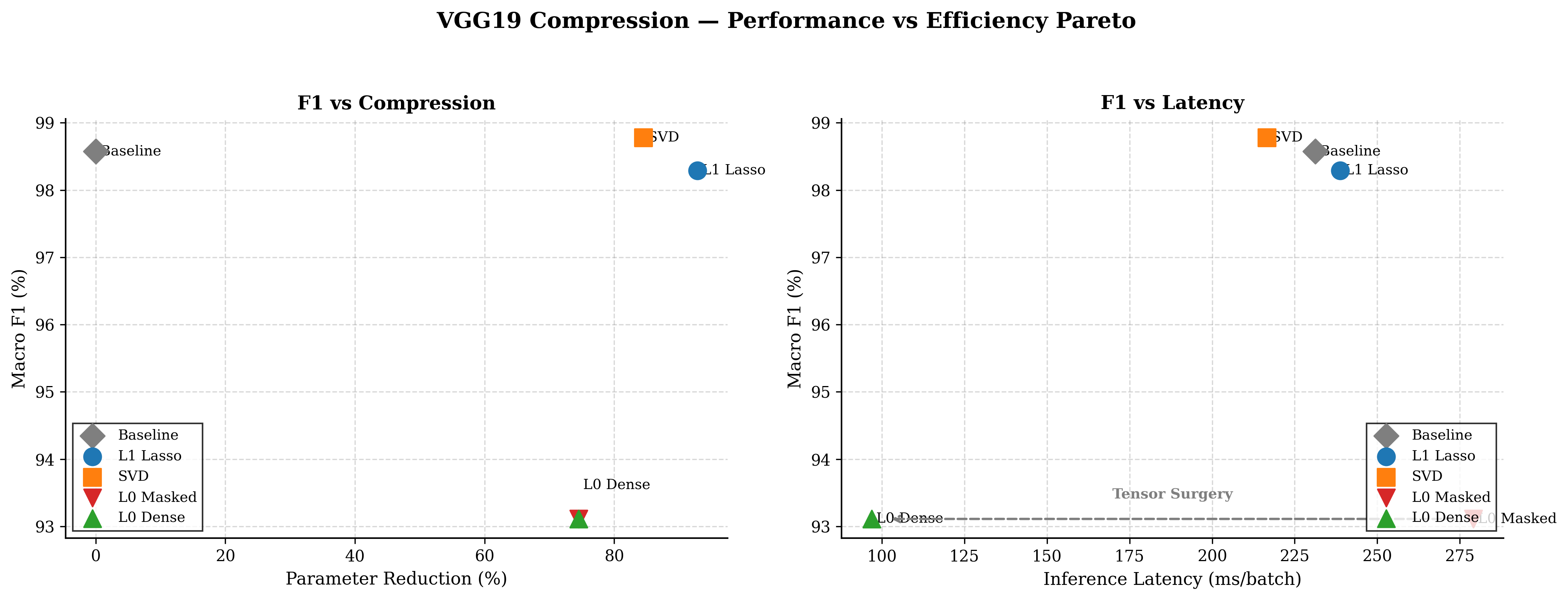
Unified predictive accuracy and performance across all compression paradigms — SVD preserves strongest aggregate F1 and ROC-AUC. L₀ variants exchange classification fidelity for structural and latency gains.
Scientific Observation Table
| Method | Active Params | Reduction | Disk Size | Memory | Latency | Speedup |
|---|---|---|---|---|---|---|
| Baseline | 139.60M | 0.0% | 532.6 MB | 3,771.7 MB | 231.3 ms | 1.000× |
| L₁ Lasso | 10.00M | 92.8% | 532.6 MB | 3,771.7 MB | 238.8 ms | 0.969× |
| SVD | 21.60M | 84.5% | 82.4 MB | 3,321.5 MB | 216.6 ms | 1.068× |
| L₀ Masked | 35.54M | 74.5% | 532.6 MB | 4,555.5 MB | 279.1 ms | 0.829× |
| L₀ Dense | 35.54M | 74.5% | 134.9 MB | 5,572.4 MB | 96.9 ms | 2.387× |
Structural compression and hardware efficiency metrics — L₀ Dense (post-surgery) is the only method achieving real wall-clock acceleration: 2.39× speedup.
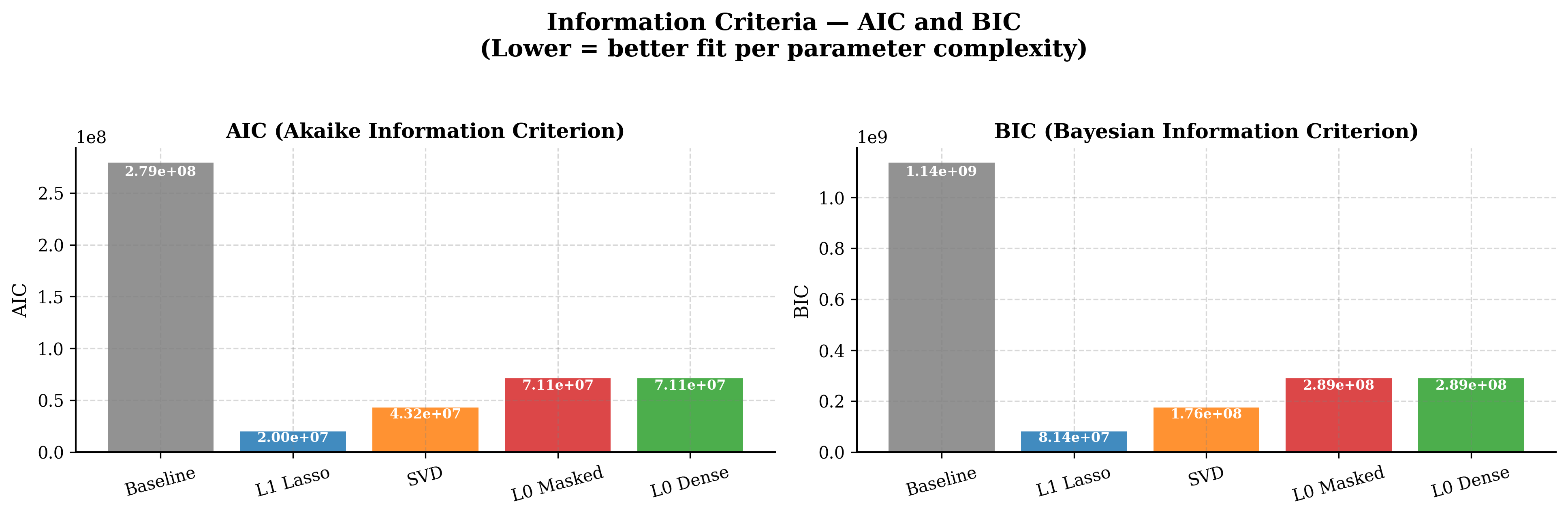
Scientific Observation Table
| Method | Log-Likelihood | AIC | BIC | LR vs Baseline |
|---|---|---|---|---|
| Baseline | −166.85 | 279,206,366 | 1,136,046,148 | Reference |
| L₁ Lasso | −193.15 | 20,000,844 | 81,379,132 | −52.60 |
| SVD | −138.27 | 43,207,077 | 175,802,009 | +57.16 |
| L₀ Dense | −809.78 | 71,089,500 | 289,247,120 | −1,285.86 |
Information-theoretic and statistical metrics — All compressed models show dramatically lower AIC/BIC than baseline, confirming severe over-parameterization. SVD uniquely improves likelihood (+57.16 LR).
The Core Hardware & Latency Paradox
We demonstrate that theoretical parameter reduction is decoupled from real-world latency acceleration. Only structured pruning with physical graph modification bypasses sparse execution bottlenecks.
Depth-Dependent Representation Survival & Clinical Guardrails
The layer survival gradient reveals that low-level visual representations are universally preserved under compression, whereas deep VGG19 layers designed for ImageNet are highly redundant for hematology.
§8. Conclusions & Recommendations
8.1 Key Findings Summary
L₁ Lasso: Statistical success, hardware failure
Achieved 92.8% unstructured sparsity with only −0.28% F1 loss. However, latency increased because tensor dimensions remained unchanged—illustrating the "ghost sparsity" paradox.
SVD: Best accuracy preservation
Reduced 84.5% of parameters while improving F1 to 98.77% (+0.20%). Compressed the model to 82.4 MB. But latency gains were modest due to kernel-dispatch overhead at extreme ranks.
L₀ + Tensor Surgery: Best deployment outcome
The only method achieving real inference speedup. Structured pruning followed by physical tensor slicing reduced latency by 50.5% (96.9 ms) while maintaining all classes above the 85% clinical guardrail.
8.2 Contributions
- Reframing compression as statistical model selection rather than heuristic engineering. The VGG19 architecture is treated as an over-parameterized non-parametric regression model.
- Unified empirical comparison of three methods under one diagnostic imaging framework, clarifying that the most sparse model ≠ fastest model ≠ best-compressed model.
- Implementation bridge from statistical sparsity to deployable inference via L₀ Gaussian gates + tensor surgery. Documentation of the “Gaussian Pivot” finding that Gaussian gates outperform Hard Concrete in pretrained transfer-learning settings.
Practitioner Implementation Recommendations
We formulate actionable engineering guidelines for deploying deep neural classifiers in clinical embedded platforms, resolving common hardware pitfalls.
Future Research Frontiers & Bayesian Compounding
Statistically guided compression opens promising development paths, including composite pruning algorithms, mixed numeric quantizations, and low-rank transformer scaling.
“The central conclusion is that statistically grounded compression can reduce deep neural network complexity substantially without sacrificing clinical utility—but only when the form of compression is aligned with the type of redundancy being removed. Compression should be treated as a criterion-specific design problem. When framed statistically, that problem becomes easier to analyze, easier to justify, and more practical to solve.”
Final Thesis Verdict
Live Diagnostic Playground
Test our regularized VGG19 models with physical channel surgery directly in the browser on the Hugging Face Spaces clinical playground.
Appendix: Hardware Stack & Reproducibility
GPU: NVIDIA T4 Tensor Core (16GB GDDR6, Turing)
CPU: Intel Xeon 2 vCPUs @ 2.20GHz
RAM: 12.7 GB System RAM
Environment: Google Colab Runtime
OS: Ubuntu 22.04 LTS
Framework: Python 3.10.x, PyTorch 2.x, CUDA 12.x
Dataset: medmnist v3.0.2, BloodMNIST+ (224px)
Inference: Batch Size 32, FP32 Precision