§6. L0 Gaussian Gating & Tensor Surgery
To achieve true hardware acceleration via structural pruning, we utilized the L0 norm—a discrete step function that strictly counts non-zero parameters. Because its derivative is identically zero everywhere, rendering standard backpropagation impossible, we bypassed traditional "Hard Concrete" approximations (which proved too violent for our pre-trained ImageNet weights, destabilizing the network).
Instead, we engineered a Gaussian Relaxation: a learnable, clamped Gaussian gate applied to every convolutional channel. By initializing the gate's mean parameter (μ = 0.5), we safely protect pre-trained features while keeping the gate only a half-step away from the pruning boundary. We then applied the Reparameterization Trick to isolate the randomness, allowing PyTorch to perfectly route gradients and train the gates.
During training, we have a tug-of-war. The Expected L0 penalty wants to increase the loss to force channels closed, while the Cross-Entropy loss wants to keep them open to maintain accuracy. We balanced them using a λ multiplier chosen automatically by a PID controller. It acted like an engine brake, controlling the sparsity until we reached equilibrium at Epoch 30. At this point, if a gate's μ parameter fell to zero, the gate closed, meaning the channel was redundant.
Interestingly, when we looked at the surviving channels, we found a Depth-Dependent Pruning Gradient. The math organically decided to keep 80% of the early layers—which detect basic edges—but aggressively deleted 80% of the deep layers, which contained useless ImageNet features.
6.5 From Ghost Sparsity to Tensor Surgery
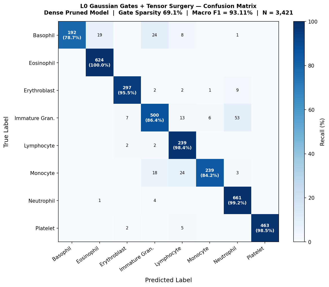
Because our dataset is imbalanced, we made sure this heavy pruning didn't just destroy our minority classes. We maintained a Macro F1 score of 93.11%, a Matthews Correlation Coefficient (MCC) of 93.00%, and a Cohen's Kappa of 92.95%.
But at this stage, we still hadn't done the real thing. We did great on paper, but in the real world, the model size was the same. We had 'Ghost Sparsity,' meaning the network was still doing the computations and multiplying weights by zero.
So, we performed Tensor Surgery. We wrote a script that checked the gates: if μ > 0, the channel remained. If μ ≤ 0, we physically sliced it out of the matrix. This shrank our model size from 532 MB down to 134.88 MB. More importantly, our latency—which is the actual wall-clock time it takes the GPU hardware to process an image—dropped to 96.9 milliseconds, making our model 50% faster.
6.6 Clinical Performance Details
Scientific Observation Table
| Cell Class | Support | F1 | Precision | Recall | AUC | Δ F1 |
|---|---|---|---|---|---|---|
| Basophil | 244 | 88.07% | 100.00% | 78.69% | 99.84% | −11.52% |
| Eosinophil | 624 | 98.42% | 96.89% | 100.00% | 99.98% | −1.50% |
| Erythroblast | 311 | 95.96% | 96.43% | 95.50% | 99.53% | −3.54% |
| Immature Gran. | 579 | 88.57% | 90.91% | 86.36% | 99.01% | −8.00% |
| Lymphocyte | 243 | 89.51% | 82.13% | 98.35% | 99.81% | −9.90% |
| Monocyte | 284 | 90.19% | 97.15% | 84.15% | 99.47% | −8.40% |
| Neutrophil | 666 | 94.90% | 90.92% | 99.25% | 99.79% | −3.60% |
| Platelet | 470 | 99.25% | 100.00% | 98.51% | 100.00% | −0.75% |
L0 per-class performance vs baseline — All classes above the 85% clinical guardrail. MCC = 93.00%, Cohen's κ = 92.95%.